Introduction to factors and directed factor graphs
We build factors up from a one-pbit sampler to directed factor graphs and composite factors. TiledFactor and ChainFactor keep the same sampling contract at each level, and deterministic same-key checks confirm they match a manual vmap and a manual feedback loop.
In this tutorial, we build the factor side of Torx from a single probabilistic bit (pbit), wire two factors into a directed factor graph, and connect that picture to the parametrised stochastic circuit (PSC) view used elsewhere in the gallery.
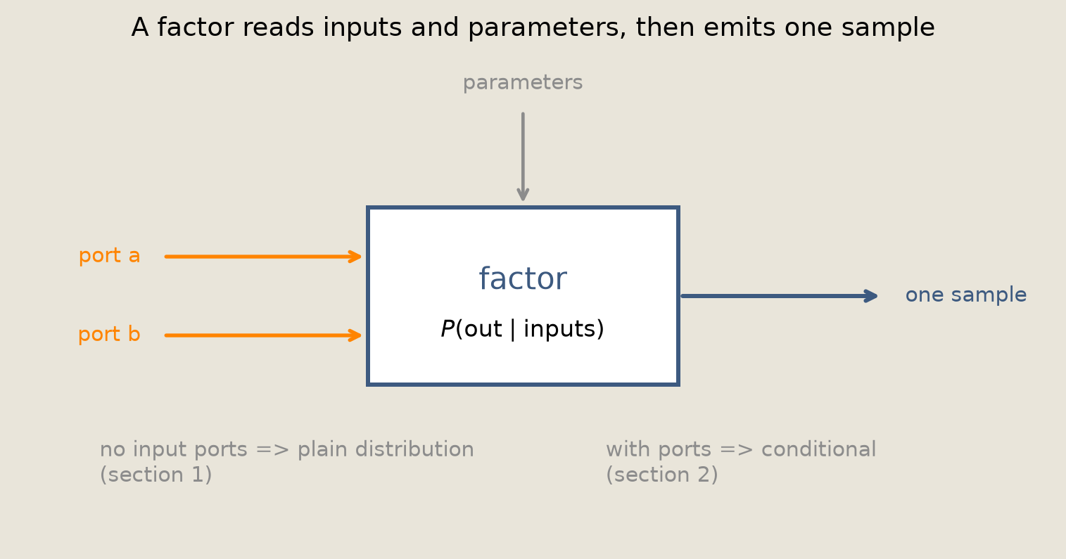
A factor is the smallest sampler on the factor side of Torx. It reads named inputs, reads parameters stored outside the object, and returns one stochastic output. A factor without inputs is a plain distribution, and its inputs, when present, are what it conditions on.
This tutorial mirrors notebook 01 from the factor side. Along the way, we add a small probabilistic dit (pdit) example with $d=3$ states for exact probabilities and connect the same ideas to the 16-spin Ising model in notebook 16.
Every gate the earlier notebooks built is already a factor. A PSWAP layer, a Gaussian gate, a MixtureGaussianGate, and an Ising spin update are all local conditional samplers wired to their neighbors, which is exactly what a factor is. A parametrised stochastic circuit is the circuit-shaped special case: those factors laid out on a fixed lattice of gates. The directed factor graph is the general object above it, any directed acyclic graph (DAG) of conditional samplers with no requirement that the wiring form a circuit. We reach it last, after fourteen circuit notebooks, because the abstraction is easiest to follow once you have built the concrete circuits it generalizes.
Setup
We set up the helper path, imports, plotting style, and figure export. The notebook's two building-block specs come next: BIT for one pbit (0 or 1) and DRIVE for a continuous value carried on an input port.
from pathlib import Path
import sys

import equinox as eqx
import jax
import jax.numpy as jnp
import numpy as np
ROOT = Path.cwd()
if not (ROOT / "helpers").exists() and (ROOT.parent / "helpers").exists():
    ROOT = ROOT.parent
HELPER_DIR = ROOT / "helpers"
sys.path.insert(0, str(HELPER_DIR))
from _notebook_paths import figure_dir
from _notebook_style import apply_notebook_style, make_savefig
import _plots_sampling as P_samp
import _plots_schematics as P_sch

from torx import (
    AbstractMatrixFactor,
    AbstractReferenceFactor,
    ChainFactor,
    DFG,
    Site,
    TiledFactor,
)
from torx.psc import JaxPRNGSampler
apply_notebook_style()
FIGURE_DIR = figure_dir(ROOT)
SEED = 16


savefig = make_savefig(FIGURE_DIR)
BIT = jax.ShapeDtypeStruct((), jnp.int32)  # one pbit, 0 or 1
DRIVE = jax.ShapeDtypeStruct((), jnp.float32)  # a continuous value on an input port
A factor as a sampler
We start with the smallest case: the CoinFactor class has no input ports, so it is just a distribution over one pbit. The parameter dictionary lives outside the object and is passed into each sample call.
The draw returns 1 with probability $\sigma(b)$.
class CoinFactor(AbstractReferenceFactor):
    """P(coin) with no inputs: one pbit drawn 1 with probability sigmoid(bias)."""

    input_ports: dict[str, jax.ShapeDtypeStruct] = eqx.field(static=True)
    output_spec: jax.ShapeDtypeStruct = eqx.field(static=True)
    sampler: JaxPRNGSampler

    def __init__(self):
        self.input_ports = {}
        self.output_spec = BIT
        self.sampler = JaxPRNGSampler()

    def init_params(self, key):
        return {"bias": jnp.array(0.4)}

    def sample(self, key, inputs, params, info=None, site_info=None, return_aux=False):
        out = self.sampler.bernoulli(key, jax.nn.sigmoid(params["bias"]))
        return (out, None) if return_aux else out
coin = CoinFactor()
coin_params = coin.init_params(jax.random.key(SEED))
keys = jax.random.split(jax.random.key(SEED + 1), 20_000)
# Many independent keys give a stable Monte Carlo estimate of the pbit mean.
coin_draws = jax.vmap(lambda k: coin.sample(k, {}, coin_params))(keys)
coin_mean = float(coin_draws.mean())
coin_target = float(jax.nn.sigmoid(coin_params["bias"]))
print(f"sampled P(coin=1) = {coin_mean:.3f}   target sigmoid(b) = {coin_target:.3f}")
sampled P(coin=1) = 0.601 target sigmoid(b) = 0.599
The sampled frequency lands on the sigmoid target, so the factor draws its declared distribution.
A factor with inputs as a conditional
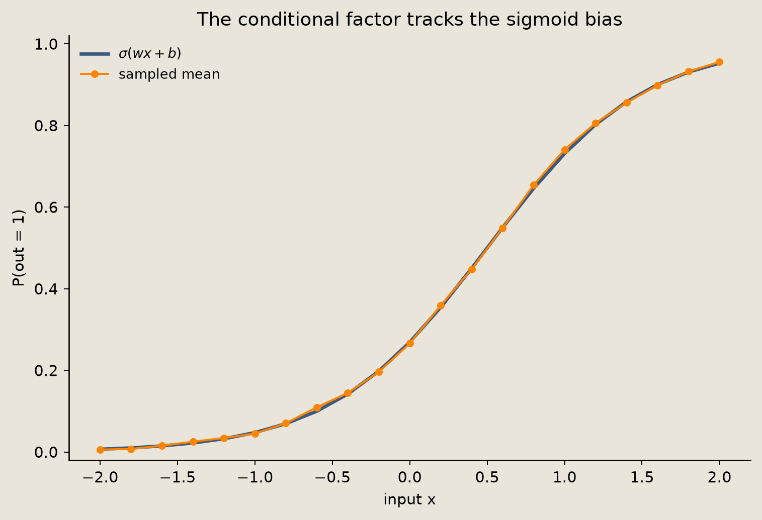
One named input port turns a sampler into a conditional.
The input arrives on the drive port, where it shifts the bit bias. We can write the conditional directly:
$$ P(\text{out}=1 \mid x) = \sigma(w x + b). $$
The sweep below checks that the sampled means track that sigmoid curve.
class ConditionalBit(AbstractReferenceFactor):
    """P(out | drive): one pbit whose bias is shifted by an input."""

    input_ports: dict[str, jax.ShapeDtypeStruct] = eqx.field(static=True)
    output_spec: jax.ShapeDtypeStruct = eqx.field(static=True)
    sampler: JaxPRNGSampler

    def __init__(self):
        self.input_ports = {"drive": DRIVE}
        self.output_spec = BIT
        self.sampler = JaxPRNGSampler()

    def init_params(self, key):
        return {"w": jnp.array(2.0), "b": jnp.array(-1.0)}

    def sample(self, key, inputs, params, info=None, site_info=None, return_aux=False):
        gamma = params["w"] * inputs["drive"] + params["b"]
        out = self.sampler.bernoulli(key, jax.nn.sigmoid(gamma))
        return (out, None) if return_aux else out
cond = ConditionalBit()
cond_params = cond.init_params(jax.random.key(SEED + 2))
xs = jnp.linspace(-2.0, 2.0, 21)
N_SWEEP = 8_000
@eqx.filter_jit
def sweep_conditional(xs, params, key):
    # (len(xs), N_SWEEP) keys: nested vmap over input points and samples,
    # one compile and no per-point host sync, then mean over the sample axis.
    """Mean conditional sample at each drive value in `xs`."""
    keys = jax.random.split(key, (xs.shape[0], N_SWEEP))

    def at_x(x, x_keys):
        draws = jax.vmap(lambda k: cond.sample(k, {"drive": x}, params))(x_keys)
        return draws.mean()

    return jax.vmap(at_x)(xs, keys)


sampled = np.asarray(sweep_conditional(xs, cond_params, jax.random.key(SEED + 3)))
exact_curve = np.asarray(jax.nn.sigmoid(cond_params["w"] * xs + cond_params["b"]))
fig = P_samp.plot_conditional_sweep(np.asarray(xs), sampled, exact_curve)
savefig(fig, "15_conditional_sweep")
Wiring two factors into a directed factor graph
A Site places a factor in a graph: it names the parents and gives a small porting function that maps parent outputs to input ports. Each Site also carries a param_key, the string src or cond here, that points to its own slice of the parameter dictionary. In the positional Site construction below, the two empty tuples after the factor are the parent list and the porting spec; a tuple of port names is an accepted porting shorthand.
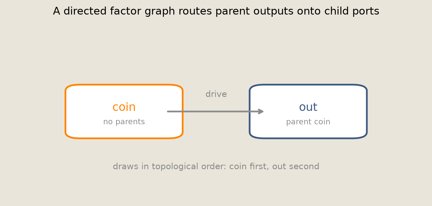
A DFG walks its sites in topological order: parents first, then the children that depend on them. Here coin draws first, and out then receives the coin bit on its drive port. The DFG itself is built from the sites, a dictionary of external input ports ({} here, since the graph takes none), and the name of the output site, "out".
A directed factor graph is itself a factor, with the same sample contract: it takes a key, the inputs, and the parameters.
The anatomy below shows that contract for a single factor: it reads any input ports and an external parameter slice, then emits one sample.
fig = P_sch.plot_factor_anatomy()
savefig(fig, "15_factor_anatomy")
def to_drive(outs):
    """Port the parent bit into the child's continuous drive input."""
    return {"drive": outs[0].astype(jnp.float32)}
sites = (
    # parentless coin: empty porting tuple, no parent outputs to route
    Site("coin", CoinFactor(), (), (), "src", info_key=None, site_info=None),
    Site(
        "out",
        ConditionalBit(),
        ("coin",),
        to_drive,
        "cond",
        info_key=None,
        site_info=None,
    ),
)
graph = DFG(sites, {}, "out")
# init_params walks the sites and returns one param slice per distinct param_key
dfg_params = graph.init_params(jax.random.key(SEED + 4))
one_draw = graph.sample(jax.random.key(SEED + 6), {}, dfg_params)
print(f"one DFG output draw: {int(one_draw)}")

keys = jax.random.split(jax.random.key(SEED + 7), 60_000)
@eqx.filter_jit
def sample_dfg_many(keys, params):
    """Draw one graph sample per key, batched under jit."""
    return jax.vmap(lambda k: graph.sample(k, {}, params))(keys)


dfg_out = sample_dfg_many(keys, dfg_params)
# Marginalize over the hidden coin by hand to check the graph sampler.
p_coin = float(jax.nn.sigmoid(dfg_params["src"]["bias"]))
w, b = dfg_params["cond"]["w"], dfg_params["cond"]["b"]
p_out_g0 = float(jax.nn.sigmoid(w * 0 + b))
p_out_g1 = float(jax.nn.sigmoid(w * 1 + b))
p_out_exact = (1 - p_coin) * p_out_g0 + p_coin * p_out_g1
p_out_emp = float(dfg_out.mean())
print(f"hand-computed P(out=1) = {p_out_exact:.3f}   sampled = {p_out_emp:.3f}")
one DFG output draw: 1
hand-computed P(out=1) = 0.546   sampled = 0.549
The sampled graph mean lands on the hand-marginalized value, so the two-node DFG composes its factors correctly. The schematic below shows the two-node graph we just sampled.
fig = P_sch.plot_two_node_dfg()
savefig(fig, "15_two_node_dfg")
Exact probabilities as an opt-in capability
Sampling is the common contract, and some finite factors can also report exact probabilities. This small example is one pdit with $d=3$ states. It implements the get_log_probability_matrix method and prints the probability table. AbstractMatrixFactor leaves sampling abstract, so this example defines both the exact matrix and the sampler. Matrix factors declare a finite state table per port, the input_states and output_states fields below, in place of the shape specs used by the factors above. Their samples come back as a dictionary keyed by output name, which is why the draws are read out with ["x"].
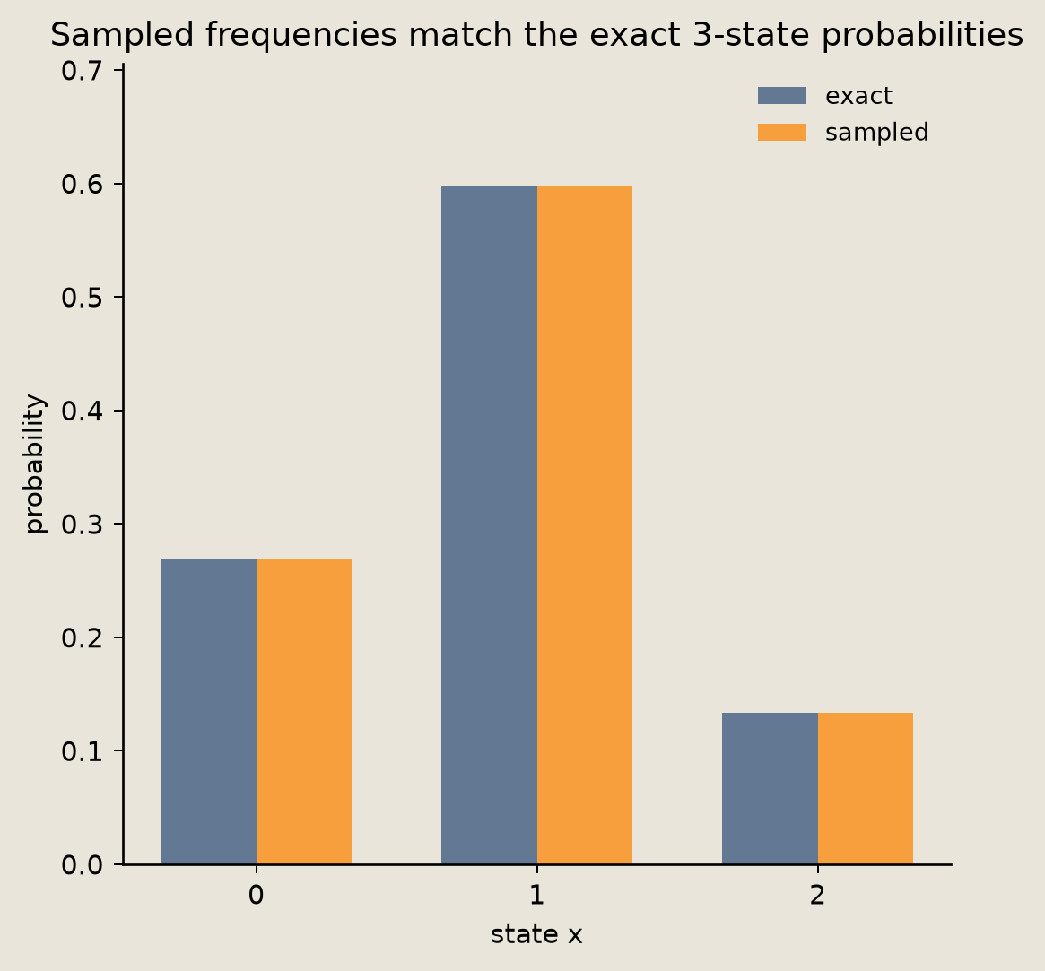
Since the factor has no inputs, the table has a single row. The comparison below puts sampled frequencies next to that exact row.
class TinyCategorical(AbstractMatrixFactor):
    """A finite 3-state pdit, no inputs, that also reports exact probabilities."""

    input_states: dict[str, jax.Array]
    output_states: dict[str, jax.Array]
    sampler: JaxPRNGSampler

    def __init__(self):
        self.input_states = {}
        self.output_states = {"x": jnp.arange(3)}
        self.sampler = JaxPRNGSampler()

    def init_params(self, key):
        return {"logits": jnp.array([0.2, 1.0, -0.5])}

    def sample(self, key, inputs, params, info=None, site_info=None, return_aux=False):
        row = self.get_log_probability_matrix(params, info, site_info)[0]
        out = self.get_nth_output_state(self.sampler.categorical(key, row))
        return (out, None) if return_aux else out

    def get_log_probability_matrix(self, params, info=None, site_info=None):
        logits = params["logits"]
        return (logits - jax.scipy.special.logsumexp(logits))[None, :]
cat = TinyCategorical()
cat_params = cat.init_params(jax.random.key(SEED + 8))
exact_p = np.asarray(jnp.exp(cat.get_log_probability_matrix(cat_params))[0])
print("exact probabilities:")
for s, p in enumerate(exact_p):
    print(f"  P(x = {s}) = {p:.3f}")
print(f"  sum        = {exact_p.sum():.3f}")

keys = jax.random.split(jax.random.key(SEED + 18), 50_000)
cat_draws = jax.vmap(lambda k: cat.sample(k, {}, cat_params))(keys)["x"]
# Compare the exact row with frequencies from many categorical draws.
emp_p = np.asarray(jax.vmap(lambda s: jnp.mean(cat_draws == s))(jnp.arange(3)))
exact probabilities:
  P(x = 0) = 0.269
  P(x = 1) = 0.598
  P(x = 2) = 0.133
  sum        = 1.000
The sampled frequencies land on the exact row, so the opt-in probability table and the sampling contract describe the same distribution. The bar chart below plots the two side by side.
fig = P_samp.plot_categorical_parity(exact_p, emp_p)
savefig(fig, "15_categorical_parity")
Copying and repeating with composite factors
Two composite factors keep common patterns short: TiledFactor runs independent copies of a factor in parallel, and ChainFactor repeats a transition and feeds the previous output back into one named input.
The feedback_porting_fn argument routes each step's output into the next step's inputs: a port-name string sends the whole output to that input. A non-feedback input is held fixed at every step. That is how notebook 16 keeps the field constant while spins evolve.
This small chain is the same object as the chain factor in notebook 16, with one pbit transition in place of a 16-spin sweep.
class FlipFactor(AbstractReferenceFactor):
    """P(next | state): a 2-state telegraph step. Input port and output are both pbits."""

    input_ports: dict[str, jax.ShapeDtypeStruct] = eqx.field(static=True)
    output_spec: jax.ShapeDtypeStruct = eqx.field(static=True)
    sampler: JaxPRNGSampler

    def __init__(self):
        self.input_ports = {"state": BIT}  # same dtype as the output: int to int
        self.output_spec = BIT
        self.sampler = JaxPRNGSampler()

    def init_params(self, key):
        return {"w": jnp.array(1.5), "b": jnp.array(0.0)}

    def sample(self, key, inputs, params, info=None, site_info=None, return_aux=False):
        gamma = params["b"] + params["w"] * (2 * inputs["state"] - 1)
        out = self.sampler.bernoulli(key, jax.nn.sigmoid(gamma))
        return (out, None) if return_aux else out
flip = FlipFactor()
flip_params = flip.init_params(jax.random.key(SEED + 9))

# parallel: 8 independent copies under one vmapped call
tiled = TiledFactor(flip, n_tiles=8, weight_tied=True)
tiled_out = tiled.sample(
    jax.random.key(SEED + 10), {"state": jnp.zeros(8, jnp.int32)}, flip_params
)

# repeat: feed the output back as the next input, 5 steps, one shared parameter set
chain = ChainFactor(flip, n_steps=5, feedback_porting_fn="state", weight_tied=True)
chain_out = chain.sample(
    jax.random.key(SEED + 11), {"state": jnp.array(0, jnp.int32)}, flip_params
)
print(f"tiled 8 parallel draws: {np.asarray(tiled_out)}")
print(f"chain after 5 steps:    {int(chain_out)}")
tiled 8 parallel draws: [1 0 0 0 1 0 1 0]
chain after 5 steps:    1
Both composites run: the tile returns eight parallel draws and the chain returns the state after five fed-back steps, each through the same sample contract as the single factor.
The factor-to-circuit ladder
The ladder is now complete. A factor is a sampler; it may be conditional, and finite factors may also be exact. A directed factor graph can be any DAG of factors sampled ancestrally. The worked example here is the two-node graph, where each node is drawn once its parent is available. The graph is itself a factor.
A PSC is the circuit-shaped specialization of the same idea, built from local gates in notebook 01.
A real model can use the factor level directly, as notebook 16 does for a 16-spin Ising model and its exact Boltzmann machine reference.
Verification
Finally, we assert the estimates computed above against their exact values, and add deterministic same-key checks for the composite factors: TiledFactor must equal a manual vmap over split keys, and ChainFactor must equal a manual loop that feeds each step's output back with the same split keys. We also compare a one-step chain against the bare factor.
COIN_MEAN_TOL = 0.02  # ~5 sigma at N=20000
COND_SWEEP_TOL = 0.03  # finite-sample
DFG_MEAN_TOL = 0.02  # finite-sample
CAT_FREQ_TOL = 0.02  # finite-sample
CHAIN_MEAN_TOL = 0.03  # finite-sample
assert abs(coin_mean - coin_target) < COIN_MEAN_TOL, (coin_mean, coin_target)
assert np.max(np.abs(sampled - exact_curve)) < COND_SWEEP_TOL
assert abs(p_out_emp - p_out_exact) < DFG_MEAN_TOL, (p_out_emp, p_out_exact)
assert abs(exact_p.sum() - 1.0) < 1e-5
assert np.max(np.abs(emp_p - exact_p)) < CAT_FREQ_TOL, (emp_p, exact_p)
# deterministic same-key check: TiledFactor == manual vmap over split keys
tiled_ref = jax.vmap(
    lambda k: flip.sample(k, {"state": jnp.array(0, jnp.int32)}, flip_params)
)(jax.random.split(jax.random.key(SEED + 10), 8))
np.testing.assert_array_equal(np.asarray(tiled_out), np.asarray(tiled_ref))
# deterministic same-key check: ChainFactor(n_steps=5) == manual feedback scan
manual_state = jnp.array(0, jnp.int32)
for step_key in jax.random.split(jax.random.key(SEED + 11), 5):
    manual_state = flip.sample(step_key, {"state": manual_state}, flip_params)
assert int(chain_out) == int(manual_state), (int(chain_out), int(manual_state))
chain1 = ChainFactor(flip, n_steps=1, feedback_porting_fn="state", weight_tied=True)
seed_state = jnp.array(0, jnp.int32)
chain_keys = jax.random.split(jax.random.key(SEED + 12), 20_000)
flip_keys = jax.random.split(jax.random.key(SEED + 13), 20_000)
chain1_draws = jax.vmap(lambda k: chain1.sample(k, {"state": seed_state}, flip_params))(
    chain_keys
)
flip_draws = jax.vmap(lambda k: flip.sample(k, {"state": seed_state}, flip_params))(
    flip_keys
)
assert abs(float(chain1_draws.mean() - flip_draws.mean())) < CHAIN_MEAN_TOL
# ChainFactor splits step keys internally.
chain_key = jax.random.key(SEED + 12)
one_step = chain1.sample(chain_key, {"state": seed_state}, flip_params)
single = flip.sample(
    jax.random.split(chain_key, 1)[0], {"state": seed_state}, flip_params
)
assert int(one_step) == int(single), (one_step, single)
print("all checks passed")
all checks passed
Conclusion
We built the factor side of Torx from one sampler up to a small directed factor graph.
A factor starts as a sampler, and input ports turn it into a conditional. Site objects wire factors into a DFG, and the graph remains a factor you can sample.
Exact probabilities are optional, and they are useful at small scale. The TiledFactor class copies a transition in parallel, while the ChainFactor class repeats it through time.
For the circuit-shaped view, go back to notebook 01. For the larger Ising model worked example, continue to notebook 16.