Simulating a regime-switching diffusion process
We control Gaussian position increments with a discrete (pdit) regime cycle to build a regime-switching diffusion sampler in which the only jumps are the latent regime switches. We check the regime-conditioned laws, the stationary occupancy, and the terminal mean against analytic references.
A regime-switching (Markov-modulated) diffusion is a continuous motion whose behavior changes when a hidden discrete state switches. In this tutorial we build one with Torx: the position $X_t$ drifts and diffuses according to a latent regime $S_t$, and only the regime jumps. Because $X_t$ has no discontinuous jump term of its own, this is a latent-jump controlled diffusion rather than a jump-diffusion in $X$.
The regime follows a discrete Markov chain. When it switches, the next position increment comes from a different Gaussian law. We assemble the two parts from PditCycle and MixtureGaussianGate. The binary-firing torx.psc.JumpDiffusionGate is a separate jump model; we do not use it here.
This pattern appears in regime-switching finance, neural spike trains, and other systems where a continuous signal changes its noise level because an unobserved state has changed. Conditioned on the current regime a Gaussian gate gives a Gaussian step, but once the regime is unobserved the same step becomes a non-Gaussian process.
The main steps are:
- advance a 3-state regime with
PditCycle, then add a regime-conditioned Gaussian step withMixtureGaussianGate, - compose the two gates into one Euler step with
HybridPCircuit, then scan it into joint discrete and continuous sample paths, and - check that the one-step law is a mixture of Gaussians, and that the long-run regime occupancy and terminal mean match the analytic references.
The same MixtureGaussianGate primitive appears in 10_pmode_gaussian_gates.ipynb, and 12_langevin_graph_ising.ipynb builds a custom nonlinear Langevin gate on the same continuous pmode site.
Setup
The setup cells wire the imports and plot styling; mixture_density, the analytic density reference used below, comes from examples/helpers/_affine_gaussian.py.
from pathlib import Path
import sys

import equinox as eqx
import jax
import jax.numpy as jnp
import numpy as np
from scipy import stats
ROOT = Path.cwd()
if not (ROOT / "helpers").exists() and (ROOT.parent / "helpers").exists():
    ROOT = ROOT.parent
HELPER_DIR = ROOT / "helpers"
sys.path.insert(0, str(HELPER_DIR))
from _notebook_paths import figure_dir
from _notebook_style import (
    apply_notebook_style,
    make_savefig,
)
import _plots_fields as P_fld
import _plots_schematics as P_sch
from _affine_gaussian import mixture_density
from torx.psc import (
    HybridPCircuit,
    HybridSampleSimulator,
    MixtureGaussianGate,
    PditCycle,
)
FIGURE_DIR = figure_dir(ROOT)
apply_notebook_style()
savefig = make_savefig(FIGURE_DIR)
SEED = 123
The process and its gates
The target is a regime-switching stochastic differential equation (SDE): a position $X_t$ whose drift and volatility are both set by a latent regime $S_t$. That regime is a continuous-time Markov chain, and PditCycle realizes its $O(\Delta t)$ Euler discretization with switch probabilities linear in $\Delta t$.
$$ dX_t = \underbrace{\mu_{S_t}\,dt}_{\vphantom{\big|}\text{drift}} + \underbrace{\sigma_{S_t}\,dW_t}_{\vphantom{\big|}\text{diffusion}}. $$
Here $W_t$ is a standard Wiener (Brownian) process, and the current regime selects $(\mu, \sigma)$ for the continuous increment.
This discrete control changes the transition kernel: the increment is Gaussian once we condition on a regime, and marginalizing over an unobserved regime turns it into a mixture of Gaussians.
The generator, the operator describing how the distribution changes over an instant, splits into a regime part and a position part, $A = A_S + A_X$. The two pieces do not commute, so the order of the approximation matters.
One Trotter step applies them in sequence: switch the regime first, then take the position step under the new regime. This is the Lie-Trotter split: its local one-step error is $O(\Delta t^2)$, giving first-order $O(\Delta t)$ global error over the full interval.
$$ T_{\text{Trotter}}(\Delta t) = \underbrace{T_{\text{MoG}}(\Delta t)}_{\vphantom{\big|}\text{position step}}\, \underbrace{T_{\text{PditCycle}}(\Delta t)}_{\vphantom{\big|}\text{regime switch}}. $$
The PditCycle gate advances the regime on a cyclic 3-state chain. At each step of size $\Delta t$ it:
- moves forward with probability $p_+ = \lambda_+\Delta t$,
- moves backward with probability $p_- = \lambda_-\Delta t$, and
- stays put with probability $p_0 = 1 - p_+ - p_-$.
The MixtureGaussianGate gate then applies the regime-conditioned increment:
$$ X' = X + \mu_k\,\Delta t + \sigma_k\sqrt{\Delta t}\,\mathcal{N}(0,1)\quad\text{when } S = k . $$
We use $K=3$ regimes with $\mu = (1.0,\,0.0,\,-0.8)$, $\sigma = (0.3,\,1.0,\,0.5)$, and rates $\lambda_+ = 0.5$ and $\lambda_- = 0.3$.
K = 3
mu = jnp.array([1.0, 0.0, -0.8])
sigma = jnp.array([0.3, 1.0, 0.5])
lambda_plus = 0.5
lambda_minus = 0.3
T = 10.0
num_steps = 120
num_trajectories = 20_000

dt = T / num_steps
# Convert continuous-time rates into one-step transition probabilities.
p_forward = lambda_plus * dt
p_backward = lambda_minus * dt
p_stay = 1.0 - p_forward - p_backward
Both gates use log-space parameters. PditCycle takes the log odds of moving forward or backward relative to staying, and MixtureGaussianGate takes per-regime means and log variances.
# PditCycle expects log odds against the stay event.
cycle_theta = jnp.log(jnp.array([p_forward / p_stay, p_backward / p_stay]))

# Each regime has its own one-dimensional Gaussian increment.
mog_theta = {
    "means": (mu * dt)[:, None],
    "log_vars": jnp.log((sigma**2 * dt)[:, None]),
}
print(
    f"dt={dt:.4f}  |  "
    f"λ+={lambda_plus}, λ-={lambda_minus}  |  "
    f"μ={mu.tolist()}  |  "
    f"σ={sigma.tolist()}  |  "
    f"trajectories={num_trajectories}"
)
print(f"p_forward={p_forward:.4f}  p_backward={p_backward:.4f}  p_stay={p_stay:.4f}")
dt=0.0833  |  λ+=0.5, λ-=0.3  |  μ=[1.0, 0.0, -0.800000011920929]  |  σ=[0.30000001192092896, 1.0, 0.5]  |  trajectories=20000
p_forward=0.0417  p_backward=0.0250  p_stay=0.9333
The regime chain
Solid edges show the forward cycle at rate $\lambda_+$, tinted by their source regime. Dashed edges show the backward cycle at rate $\lambda_-$ in a single neutral color. The self-loops for the stay probability $p_0$ are omitted so the drawing focuses on transitions between regimes.
Because the chain is rotationally symmetric, its stationary distribution, the long-run fraction of time spent in each regime, is uniform $(1/3, 1/3, 1/3)$ for any split between the forward and backward rates. The occupancy check at the end confirms this empirically.
fig_g = P_sch.draw_regime_chain(
    mu=mu,
    lambda_plus=lambda_plus,
    lambda_minus=lambda_minus,
)
savefig(fig_g, "13_regime_transition_graph")
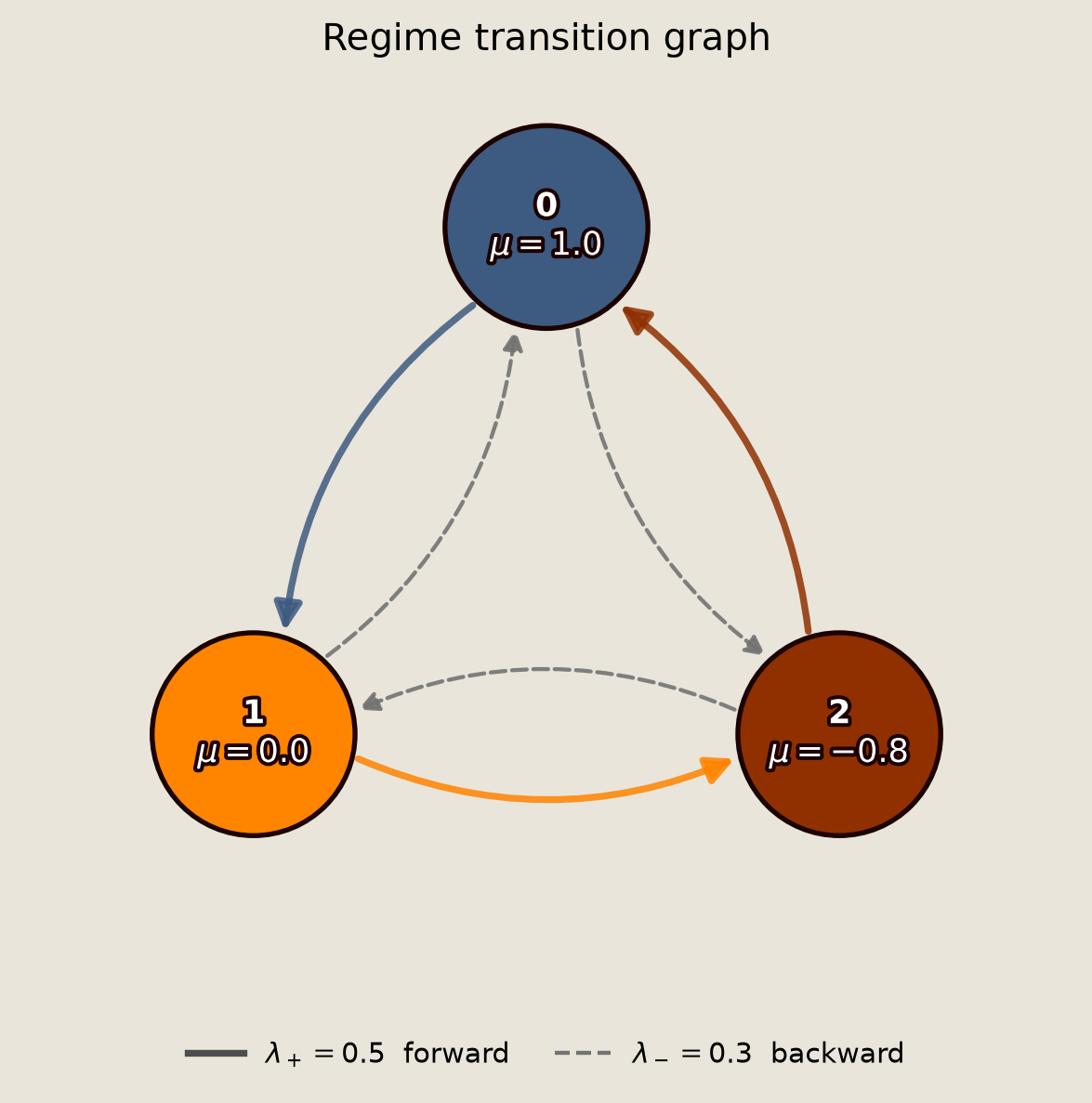
Every switch is a single forward or backward step around the ring. For $K=3$ both non-self states are nearest neighbors, so one step can reach either. On larger rings this would permit only nearest-neighbor moves.
Building the one-step circuit
We use the Trotter split $T_{\text{Trotter}} = T_{\text{MoG}}\,T_{\text{PditCycle}}$ to update the regime wire $|S)$ first. The Gaussian gate then samples the position increment on the wire $|X)$, conditioned on the new regime.
one_step = HybridPCircuit(
    [
        PditCycle(sites=0, dims=K),
        MixtureGaussianGate(sites=(0, 0), dims=(1,), num_components=K),
    ]
)

# Parameters are kept separate from the circuit, one pytree per gate in gate order.
thetas = [cycle_theta, mog_theta]
fig_c = P_sch.draw_pcircuit(
    # MoG spans both wires: it reads the regime wire 0 and writes the position wire 1
    [("PditCycle", [0]), ("MoG", [0, 1])],
    wire_labels=[r"$|S)$ regime", r"$|X)$ position"],
    title="One regime-switching step",
)
savefig(fig_c, "13_one_step_circuit")
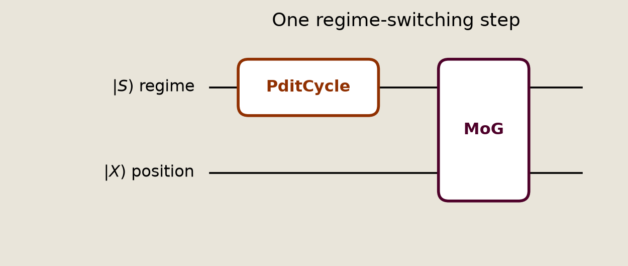
The regime wire $|S)$ is updated before it conditions the Gaussian increment on $|X)$, so each step samples the position under the freshly switched regime.
Scanning the trajectories
The HybridSampleSimulator class runs one path at a time with num_samples set to 1.
sim = HybridSampleSimulator(num_samples=1)
compiled = sim.build_circuit(one_step, thetas)
The scan function carries the discrete and continuous state through each compiled step. The vmap transform then batches the 20,000 trajectory keys into one compiled computation.
@eqx.filter_jit
def simulate_trajectories(keys):
    def simulate_one(key):
        # Split once so every timestep gets an independent random key.
        step_keys = jax.random.split(key, num_steps)
        init = {
            "discrete": jnp.array([0], dtype=jnp.int32),
            "continuous": jnp.zeros(1),
        }

        def step(state, step_key):
            result = sim.sample(compiled, state, step_key)
            sampled_discrete = result["discrete"][0]
            sampled_continuous = result["continuous"][0]
            new_state = {
                "discrete": sampled_discrete,
                "continuous": sampled_continuous,
            }
            # why: num_samples=1 leaves a leading axis; carry drops it and scan stores scalars.
            return new_state, (sampled_discrete[0], sampled_continuous[0])

        _, path = jax.lax.scan(step, init, step_keys)
        return path

    return jax.vmap(simulate_one)(keys)
keys = jax.random.split(jax.random.key(SEED), num_trajectories)
regimes, positions = simulate_trajectories(keys)

regimes = np.asarray(regimes)
positions = np.asarray(positions)

# prepend the initial state (t=0, regime 0, position 0) so occupancy and path
# plots start at t=0, before the first PditCycle transition
init_regime = np.zeros((num_trajectories, 1), dtype=regimes.dtype)
init_position = np.zeros((num_trajectories, 1), dtype=positions.dtype)
regimes = np.concatenate([init_regime, regimes], axis=1)
positions = np.concatenate([init_position, positions], axis=1)
time = np.linspace(0.0, T, num_steps + 1)

assert regimes.shape == (num_trajectories, num_steps + 1), regimes.shape
assert positions.shape == (num_trajectories, num_steps + 1), positions.shape
assert set(np.unique(regimes)).issubset(set(range(K))), "invalid regime index"
assert np.all(np.isfinite(positions)), "non-finite positions"

print(
    f"regimes shape: {regimes.shape}   positions shape: {positions.shape}\n"
    f"regime values present: {sorted(np.unique(regimes).tolist())}\n"
    f"position range: [{positions.min():.2f}, {positions.max():.2f}]"
)
regimes shape: (20000, 121)   positions shape: (20000, 121)
regime values present: [0, 1, 2]
position range: [-12.21, 14.83]
The one-step transition density
One application of PditCycle followed by MixtureGaussianGate produces a Gaussian mixture.
Conditioning on the new regime $k$ gives the Gaussian increment $\mathcal{N}(\mu_k\Delta t,\,\sigma_k^2\Delta t)$. Marginalizing over regimes (averaging across all possible regimes) with the stationary weights $\pi = (1/3, 1/3, 1/3)$ gives $\Delta x \sim \sum_k \pi_k\,\mathcal{N}(\mu_k\Delta t,\,\sigma_k^2\Delta t)$.
The pooled sample below starts equally often from each regime. Because this PditCycle chain is doubly stochastic (rows and columns each sum to 1), that uniform start remains uniform after one step, so pooling per-regime samples reproduces the stationary marginal.
The discrete control is what makes the kernel non-Gaussian; compositions of pure-Gaussian gates stay Gaussian.
As a check, we sample the one-step increments $\Delta x$ from each starting regime and compare them with the analytic densities.
N_PER_REGIME = 20_000
sim_one = HybridSampleSimulator(num_samples=N_PER_REGIME)
compiled_one = sim_one.build_circuit(one_step, thetas)
def sample_one_step_by_regime(sim_one, compiled_one, K, seed):
    """Sample one circuit step started from each regime; return new regimes and increments."""
    new_regimes_list, increments_list = [], []
    base_key = jax.random.key(seed)
    for start_regime in range(K):
        # Start equally from each regime; samples are grouped by the new regime
        # S_{n+1} below, so the conditional laws are conditioned on S_{n+1}.
        init_state = {
            "discrete": jnp.array([start_regime], dtype=jnp.int32),
            "continuous": jnp.zeros(1),
        }
        samples_k = sim_one.sample(
            compiled_one,
            init_state,
            jax.random.fold_in(base_key, start_regime),
        )
        new_regimes_list.append(np.asarray(samples_k["discrete"])[:, 0])
        increments_list.append(np.asarray(samples_k["continuous"])[:, 0])

    all_new_regimes = np.concatenate(new_regimes_list)
    all_increments = np.concatenate(increments_list)
    return all_new_regimes, all_increments
all_new_regimes, all_increments = sample_one_step_by_regime(
    sim_one,
    compiled_one,
    K,
    SEED,
)

print(
    f"{K * N_PER_REGIME} total samples; new-regime counts: "
    f"{[int((all_new_regimes == k).sum()) for k in range(K)]}"
)
60000 total samples; new-regime counts: [20010, 19984, 20006]
conditional_increments = [all_increments[all_new_regimes == k] for k in range(K)]
marginal_increments = all_increments
pi_stat = np.full(K, 1.0 / K)

regime_means = np.asarray(mu * dt)
regime_vars = np.asarray(sigma**2 * dt)

print("regime  mean(Δx)   var(Δx)")
for k in range(K):
    print(f"  {k}     {regime_means[k]:+.4f}    {regime_vars[k]:.4f}")
regime  mean(Δx)   var(Δx)
  0     +0.0833    0.0075
  1     +0.0000    0.0833
  2     -0.0667    0.0208
We evaluate the analytic conditional and mixture densities on a shared grid with the mixture_density helper, then overlay them on the sampled histograms.
# A shared grid makes the conditional and marginal curves directly comparable.
x_lo = regime_means.min() - 4.0 * np.sqrt(regime_vars.max())
x_hi = regime_means.max() + 4.0 * np.sqrt(regime_vars.max())
x_grid = np.linspace(x_lo, x_hi, 400)
conditional_pdfs = [
    np.asarray(
        mixture_density(
            mog_theta["means"][k : k + 1],
            mog_theta["log_vars"][k : k + 1],
            jnp.array([1.0]),
            jnp.asarray(x_grid),
        )
    )
    for k in range(K)
]
marginal_pdf = np.asarray(
    mixture_density(
        mog_theta["means"],
        mog_theta["log_vars"],
        jnp.asarray(pi_stat),
        jnp.asarray(x_grid),
    )
)
fig = P_fld.plot_transition_density(
    conditional_increments,
    marginal_increments,
    x_grid,
    conditional_pdfs,
    marginal_pdf,
)
savefig(fig, "13_mog_transition_density")
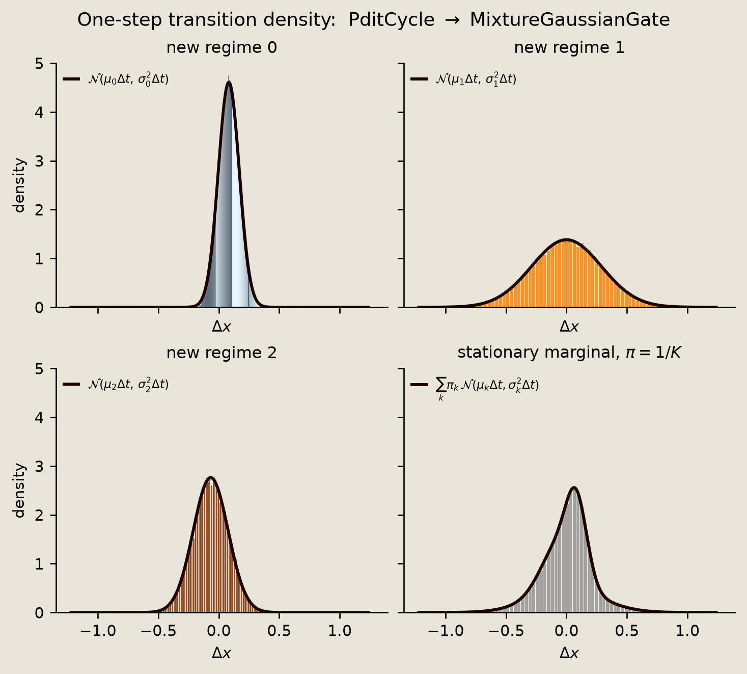
Regimes 0 and 2 give narrow conditional Gaussians, while regime 1 gives a wide one. The stationary marginal blends all three, so it is wider than the sharpest conditional.
Sample-law checks
The exact target law lets us check the full distribution.
Each regime-conditional increment is $\mathcal{N}(\mu_k\Delta t,\sigma_k^2\Delta t)$, and the stationary marginal is the mixture $\sum_k \pi_k\,\mathcal{N}(\mu_k\Delta t,\sigma_k^2\Delta t)$.
The Kolmogorov-Smirnov (KS) statistic measures the largest gap between the empirical and true cumulative distribution function (CDF), where 0 is perfect.
The checks below report KS D per regime and for the stationary marginal, then verify the sample means and variances against the analytic moments.
def ks_statistic(samples, cdf):
    # KS D straight from the empirical vs theoretical CDF, bypassing scipy's KS
    # wrapper (its _axis_nan_policy path regressed on scipy 1.18); norm.cdf is fine.
    xs = np.sort(np.asarray(samples, dtype=float))
    n = len(xs)
    cdf_vals = np.asarray(cdf(xs), dtype=float)
    d_plus = np.max(np.arange(1, n + 1) / n - cdf_vals)
    d_minus = np.max(cdf_vals - np.arange(0, n) / n)
    return float(max(d_plus, d_minus))
def mixture_cdf(x):
    """Stationary-mixture CDF of the one-step increment."""
    return sum(
        pi_stat[k] * stats.norm.cdf(x, regime_means[k], np.sqrt(regime_vars[k]))
        for k in range(K)
    )
print("target                         KS D")
ks_stats = []
for k in range(K):
    inc = conditional_increments[k]
    loc, scale = regime_means[k], float(np.sqrt(regime_vars[k]))
    D = ks_statistic(inc, lambda x, loc=loc, scale=scale: stats.norm.cdf(x, loc, scale))
    ks_stats.append(D)
    print(f"  Δx | new regime = {k}         {D:.4f}")

D_mix = ks_statistic(marginal_increments, mixture_cdf)
ks_stats.append(D_mix)
print(f"  Δx  (stationary mixture)       {D_mix:.4f}")

min_ks_samples = min([len(inc) for inc in conditional_increments] + [len(marginal_increments)])
ks_tol = 5.0 / np.sqrt(min_ks_samples)
# why: KS sampling error falls as 1/sqrt(n).
if max(ks_stats) >= ks_tol:
    raise AssertionError(
        f"KS D too large: {max(ks_stats):.4f} >= {ks_tol:.4f} "
        "(increments not matching the law)"
    )
print(
    f"\nall KS D < {ks_tol:.4f}; one-step increments match the analytic transition law"
)
target                         KS D
  Δx | new regime = 0         0.0060
  Δx | new regime = 1         0.0051
  Δx | new regime = 2         0.0101
  Δx  (stationary mixture)       0.0036

all KS D < 0.0354; one-step increments match the analytic transition law
for k in range(K):
    inc_k = conditional_increments[k]
    if len(inc_k) <= 100:
        raise AssertionError(f"too few samples for regime {k}")
    mean_atol = 7.0 * np.sqrt(regime_vars[k] / len(inc_k))
    var_rtol = 10.0 * np.sqrt(2.0 / (len(inc_k) - 1))
    np.testing.assert_allclose(inc_k.mean(), regime_means[k], atol=mean_atol)
    np.testing.assert_allclose(inc_k.var(), regime_vars[k], rtol=var_rtol)
mix_mean_exact = float((pi_stat * regime_means).sum())
mix_var_exact = float(
    (pi_stat * (regime_vars + regime_means**2)).sum() - mix_mean_exact**2
)
marginal_mean_atol = 7.0 * np.sqrt(mix_var_exact / len(marginal_increments))
marginal_var_rtol = 10.0 * np.sqrt(2.0 / (len(marginal_increments) - 1))
np.testing.assert_allclose(
    marginal_increments.mean(), mix_mean_exact, atol=marginal_mean_atol
)
np.testing.assert_allclose(marginal_increments.var(), mix_var_exact, rtol=marginal_var_rtol)
print("per-regime Torx moments match analytic to MC tolerance.")
print(
    f"stationary marginal:  Torx mean = {marginal_increments.mean():+.4f}, "
    f"analytic = {mix_mean_exact:+.4f}"
)
print(
    f"stationary marginal:  Torx var  = {marginal_increments.var():.4f}, "
    f"analytic = {mix_var_exact:.4f}"
)
per-regime Torx moments match analytic to MC tolerance.
stationary marginal:  Torx mean = +0.0066, analytic = +0.0056
stationary marginal:  Torx var  = 0.0410, analytic = 0.0410
Sample paths
The sampled trajectories show how regime changes alter the continuous motion.
The figure shows 18 paths, with each segment colored by its active regime. A color change along a path marks a regime jump. Slate is regime 0 with upward drift $\mu=1.0$, orange is regime 1 with pure diffusion $\mu=0.0$, and copper is regime 2 with downward drift $\mu=-0.8$.
fig = P_fld.plot_sample_paths(time, positions, regimes, mu=mu, sigma=sigma, n_show=18)
savefig(fig, "13_regime_switching_diffusion_trajectories")
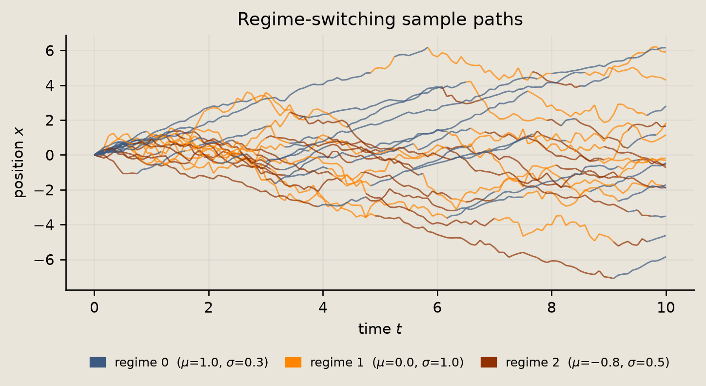
In the color bands, slate segments drift up, copper segments drift down, and orange segments wander widest. The active regime sets both the direction and the spread of every increment.
Regime occupancy
Regime occupancy summarizes how the discrete chain mixes.
At each timestep, occupancy is the fraction of paths in each regime. The three stacked bands sum to 1 at every $t$. All paths start in regime 0, so the bands begin with all mass in that regime and then relax toward the uniform stationary distribution $(1/3, 1/3, 1/3)$.
occupancy = np.stack([(regimes == k).mean(axis=0) for k in range(K)])

np.testing.assert_allclose(occupancy.sum(axis=0), 1.0, atol=1e-6)
print("regime occupancy sums to 1 at every step")
print(f"time-mean occupancies: {occupancy.mean(axis=1).round(3).tolist()}")
regime occupancy sums to 1 at every step
time-mean occupancies: [0.388, 0.313, 0.299]
fig = P_fld.plot_regime_occupancy(time, occupancy)
savefig(fig, "13_regime_switching_diffusion_regime_histogram")
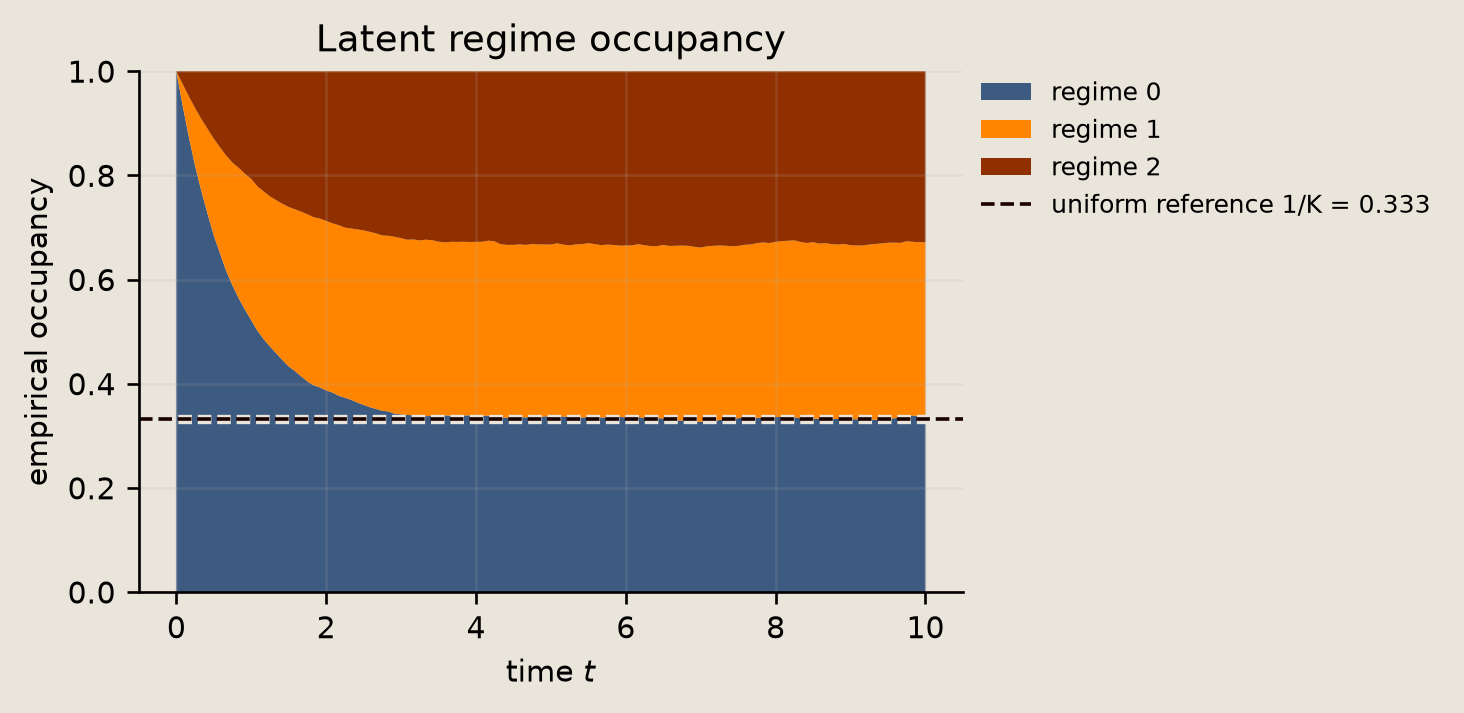
The regime-0 band falls from 1 and the other two rise. Once the chain forgets its start, all three settle near $1/3$.
Verification
Two quantitative checks close the notebook.
First, the back-half time-mean occupancy across the sampled paths should reach the uniform stationary distribution $(1/3, 1/3, 1/3)$ once the chain has mixed.
Second, the empirical terminal $E[x_T]$ should match the analytic per-step mean propagation.
First we check that the back-half occupancy has reached the uniform stationary distribution.
uniform_stationary = np.full(K, 1.0 / K)
back_half_occupancy = occupancy[:, num_steps // 2 :].mean(axis=1)
max_dev_back = float(np.max(np.abs(back_half_occupancy - uniform_stationary)))

# why: paths are independent, while back-half time points are correlated.
occupancy_tol = 1.35 / np.sqrt(num_trajectories)

print(
    f"back-half occupancy (mean for t > T/2): {back_half_occupancy.round(4).tolist()}"
)
print(f"uniform stationary  (1/K, 1/K, 1/K):    {uniform_stationary.round(4).tolist()}")
print(f"max |empirical - stationary|:           {max_dev_back:.4f}  (tol {occupancy_tol:.4f})")
if max_dev_back >= occupancy_tol:
    raise AssertionError(
        f"back-half occupancy deviates from uniform stationary by {max_dev_back:.4f} "
        f">= {occupancy_tol:.4f}; chain may not be mixed or sample count too small"
    )
back-half occupancy (mean for t > T/2): [0.3339, 0.3341, 0.332]
uniform stationary  (1/K, 1/K, 1/K):    [0.3333, 0.3333, 0.3333]
max |empirical - stationary|:           0.0014  (tol 0.0095)
Then we propagate the regime distribution through the transition matrix to get the analytic terminal mean and compare it with the empirical one.
T_matrix = np.asarray(PditCycle(sites=0, dims=K).get_matrix(cycle_theta))
regime_dist = np.array([1.0, 0.0, 0.0])
analytic_terminal_mean = 0.0
for _ in range(num_steps):
    # why: Torx uses column-stochastic p_next = T @ p, matching the sampler.
    regime_dist = T_matrix @ regime_dist
    analytic_terminal_mean += float((regime_dist * np.asarray(mu)).sum()) * dt

empirical_terminal_mean = float(positions[:, -1].mean())
empirical_terminal_sem = float(positions[:, -1].std(ddof=1) / np.sqrt(num_trajectories))

print()
print(
    f"terminal E[x_T]:  analytic = {analytic_terminal_mean:+.4f}, "
    f"empirical = {empirical_terminal_mean:+.4f}  "
    f"(SE {empirical_terminal_sem:.3f} from {num_trajectories} paths)"
)

# why: terminal mean error is Monte Carlo standard error over independent paths.
terminal_tol = 4.0 * empirical_terminal_sem
if abs(empirical_terminal_mean - analytic_terminal_mean) >= terminal_tol:
    raise AssertionError(
        f"terminal mean off by {empirical_terminal_mean - analytic_terminal_mean:+.4f} "
        f"(tolerance ±{terminal_tol:.3f})"
    )
terminal E[x_T]: analytic = +1.4052, empirical = +1.4295 (SE 0.024 from 20000 paths)
The empirical terminal mean lands within four standard errors of the analytic propagation; the summary below collects the run statistics.
print()
print(f"Regime-switching diffusion  (K=3 regimes, 120 steps, {num_trajectories} paths)")
print(f"  position range          : [{positions.min():+.3f}, {positions.max():+.3f}]")
print(f"  terminal mean (empir.)  : {empirical_terminal_mean:+.4f}")
print(f"  terminal mean (analytic): {analytic_terminal_mean:+.4f}")
print(f"  time-mean occupancy     : {occupancy.mean(axis=1).round(4).tolist()}")
print(f"  back-half occupancy     : {back_half_occupancy.round(4).tolist()}")
print(f"  occupancy vs stationary : max dev {max_dev_back:.4f}")
Regime-switching diffusion  (K=3 regimes, 120 steps, 20000 paths)
  position range          : [-12.215, +14.826]
  terminal mean (empir.)  : +1.4295
  terminal mean (analytic): +1.4052
  time-mean occupancy     : [0.3881, 0.3132, 0.2987]
  back-half occupancy     : [0.3339, 0.3341, 0.332]
  occupancy vs stationary : max dev 0.0014
Conclusion
We built a regime-switching diffusion where a pdit-controlled Gaussian mixture gate turns a Gaussian step into a non-Gaussian marginal.
PditCycle advances the 3-state regime chain with first-order transition probabilities, and MixtureGaussianGate draws the regime-conditioned position increment. HybridPCircuit composes the gates into one Euler step, and a jit-compiled scan and vmap around HybridSampleSimulator run 20,000 paths over 120 steps.
The one-step transition density is a mixture of Gaussians that matches the analytic conditionals and the stationary marginal under the uniform, doubly stochastic regime law. The final checks show that the back-half regime occupancy reaches the uniform stationary distribution, and that the empirical terminal $E[x_T]$ matches the analytic mean propagation.
See also:
10_pmode_gaussian_gates.ipynb, pure affine-Gaussian gates and exact moment propagation.12_langevin_graph_ising.ipynb, a custom nonlinear Langevin gate sampling a soft-spin energy.