Sampling Langevin dynamics on a graph Ising model
We sample the continuous Boltzmann law of a soft-spin graph Ising energy with a custom overdamped-Langevin LangevinGate driven by HybridSampleSimulator. We validate the Metropolis-adjusted (MALA) chain against exact quadrature and compare it with the unadjusted (ULA) chain.
Overdamped Langevin dynamics is noisy gradient descent on an energy. Repeating the step $x \leftarrow x - \varepsilon\,\nabla V(x) + \sqrt{2T\varepsilon}\,\xi$ with $\xi\sim\mathcal N(0,I)$ drives the state toward the Boltzmann law $\pi(x)\propto e^{-V(x)/T}$: samples concentrate where the energy $V$ is low, with spread set by the temperature $T$.
Each node of a graph carries a real-valued soft spin. Neighboring nodes nudge each other toward alignment while an external field tilts the pattern, so this is a continuous-variable cousin of an Ising sampler.
In this tutorial, we sample that Boltzmann law with LangevinGate, custom notebook code built on Torx's AbstractContinuousGate interface and defined in the helper module examples/helpers/_langevin.py, shown below. Its sample method takes one gradient-drift step on the soft-spin energy. We drive it with HybridSampleSimulator in two modes, unadjusted (ULA) and Metropolis-adjusted (MALA); the gate section below spells out the difference.
Because the drift $\nabla V$ is nonlinear, this gate has no closed-form affine-Gaussian channel, so we cannot read off exact Gaussian moments the way a linear gate allows. Instead we validate the sampler where the target is tractable, a one-dimensional instance of the same energy whose Boltzmann density we obtain by fine-grid quadrature, and then deploy that same gate on the full graph.
The main steps are:
- define the soft-spin Ising energy $V$ (continuous spins instead of hard plus or minus one) on a 10-node graph,
- build the custom
LangevinGate(ULA and MALA) and sample it withHybridSampleSimulator, - validate MALA against exact quadrature on a tractable 1-D instance and expose ULA's step-size bias, and
- deploy the validated MALA gate on the full graph and read off its equilibrium soft-spin field, magnetization, and energy.
This example is the continuous-state companion to the discrete graph notebooks earlier in the series.
Setup
The setup cells wire the import path and plot styling; LangevinGate and its validation utilities come from the helper module examples/helpers/_langevin.py.
from pathlib import Path
import sys

import equinox as eqx
import jax
import jax.numpy as jnp
import networkx as nx
import numpy as np

from torx.psc import HybridPCircuit, HybridSampleSimulator
ROOT = Path.cwd()
if not (ROOT / "helpers").exists() and (ROOT.parent / "helpers").exists():
    ROOT = ROOT.parent
HELPER_DIR = ROOT / "helpers"
sys.path.insert(0, str(HELPER_DIR))

from _notebook_paths import figure_dir
from _notebook_style import (
    apply_notebook_style,
    display_and_close,
    make_savefig,
)
from _langevin import (
    LangevinGate,
    boltzmann_1d_reference,
    ks_distance,
    langevin_theta,
    plot_ks_vs_step,
    plot_mala_reference,
    plot_site_mean_parity,
    plot_ula_bias,
)
import _plots_sampling as P_samp
import _plots_schematics as P_sch
FIGURE_DIR = figure_dir(ROOT)
apply_notebook_style()

SEED = 31

savefig = make_savefig(FIGURE_DIR)
The graph and soft-spin Ising energy
The target is a 10-node graph: a cycle plus three cross-chords.
That geometry fixes the soft-spin Ising energy. Each node carries a soft spin $s_i = \tanh(x_i)$, $A_{\mathrm{adj}}$ is the adjacency matrix, and
$$V(x) = \underbrace{-\frac{\beta}{2}\, s^\top A_{\mathrm{adj}}\, s}_{\vphantom{\big|}\text{bond energy}} \;-\; h^\top s \;+\; \underbrace{\frac{\lambda_q}{4}\sum_i (x_i^2 - 1)^2}_{\vphantom{\big|}\text{spin well}}, \qquad s_i = \tanh(x_i).$$
The bond term rewards aligned neighbors, the field term $-h^\top s$ tilts the pattern, and the quartic well softly confines each coordinate near $x_i = \pm 1$.
This $V$ is the potential the gate descends, and its Boltzmann law $\pi(x)\propto e^{-V(x)/T}$ is the distribution we sample.
We now build the graph and field that define the system.
graph = nx.cycle_graph(10)
# Add three long-range chords so the cycle has nonlocal couplings.
graph.add_edges_from([(0, 5), (2, 7), (3, 8)])
pos = nx.spring_layout(graph, seed=SEED)

n = graph.number_of_nodes()
adj = nx.to_numpy_array(graph, dtype=float)
# Antisymmetric field: a per-site tilt from negative to positive that sums to ~0.
field = np.linspace(-0.30, 0.30, n)
assert graph.number_of_nodes() == 10
assert graph.number_of_edges() == 13  # 10 cycle edges + 3 cross-chords
print(f"graph: {n} nodes, {graph.number_of_edges()} edges")
graph: 10 nodes, 13 edges
The Langevin gate
LangevinGate is custom notebook code rather than a Torx API class. It implements the AbstractContinuousGate interface and ships with the notebooks; at run time the simulator passes each gate's theta to sample as params. The following is excerpted from examples/helpers/_langevin.py:
class LangevinGate(AbstractContinuousGate[dict[str, Array], tuple[int, ...]]):
    ...
    metropolis: bool = eqx.field(static=True, default=False)

    def energy(
        self, x: Float[Array, " d"], theta: dict[str, Array]
    ) -> Float[Array, ""]:
        """Soft-spin quartic Ising energy $V(x)$ that the gate descends."""
        s = jnp.tanh(x)
        coupling = -0.5 * theta["beta"] * (s @ (theta["adj"] @ s))
        bias = -(theta["field"] @ s)
        quartic = 0.25 * theta["lam_quartic"] * jnp.sum((x * x - 1.0) ** 2)
        return coupling + bias + quartic

    def sample(
        self,
        key: Key[Array, ""],
        inputs: Mapping[str, PyTree[Array]],
        params: dict[str, Array],
        ...
    ):
        """Advance the continuous state by one (optionally adjusted) Langevin step."""
        x = inputs["continuous"]
        eps = params["step"]
        temperature = params["temperature"]
        grad_x = jax.grad(self.energy)(x, params)

        noise_key, accept_key = jax.random.split(key)
        ...
            noise = jax.random.normal(noise_key, x.shape, dtype=x.dtype)
        ...

        proposal = x - eps * grad_x + jnp.sqrt(2.0 * temperature * eps) * noise

        if not self.metropolis:
            output = proposal
        else:
            grad_prop = jax.grad(self.energy)(proposal, params)
            # log target ratio: -(V(x') - V(x)) / T
            log_target = (
                -(self.energy(proposal, params) - self.energy(x, params)) / temperature
            )
            # log proposal ratio log q(x | x') - log q(x' | x); the Gaussian
            # proposal has mean y - eps * grad V(y) and covariance 2 T eps I.
            fwd = proposal - (x - eps * grad_x)
            bwd = x - (proposal - eps * grad_prop)
            log_proposal = (jnp.sum(fwd**2) - jnp.sum(bwd**2)) / (
                4.0 * temperature * eps
            )
            accept_prob = jnp.exp(jnp.minimum(0.0, log_target + log_proposal))
            ...
                accepted = jax.random.bernoulli(accept_key, accept_prob)
            ...
            output = jnp.where(accepted, proposal, x)
sample takes one overdamped-Langevin step on the soft-spin energy above:
$$x' = x \underbrace{-\,\varepsilon\,\nabla V(x)}_{\vphantom{\big|}\text{gradient drift}} + \underbrace{\sqrt{2T\varepsilon}\,\xi}_{\vphantom{\big|}\text{Gaussian noise}},\qquad \xi\sim\mathcal N(0, I).$$
The gradient $\nabla V$ is jax.grad applied to the gate's own energy method, so the gate descends the same energy it defines. Repeating the step drives the chain toward $\pi(x)\propto e^{-V(x)/T}$. The structural metropolis flag selects between two modes:
- ULA (
metropolis=False) returns the raw proposal. Discretizing the continuous dynamics leaves an $O(\varepsilon)$ bias, so ULA samples a slightly wrong distribution. - MALA (
metropolis=True) accepts the proposal with the Metropolis-Hastings probability for $\pi$ and otherwise stays put. The accept/reject step cancels the discretization bias, so MALA is asymptotically exact for $e^{-V/T}$.
The energy coefficients and integrator constants travel in theta, exactly as AffineGaussianGate carries its $(A, b, \log\mathrm{var})$: adj, field, beta, lam_quartic, step ($\varepsilon$), and temperature ($T$). Below we set the deploy-time constants and pack them into theta with the langevin_theta helper.
BETA = 0.35
LAM_QUARTIC = 0.6
STEP_SIZE = 0.04
TEMPERATURE = 0.35

DEPLOY_REPS = 1200     # Metropolis-adjusted steps per deployed chain
LONGRUN_REPS = 6000    # a much longer MALA run, used as a convergence reference
NUM_SAMPLES = 1024
theta = langevin_theta(
    adj=adj,
    field=field,
    beta=BETA,
    lam_quartic=LAM_QUARTIC,
    step=STEP_SIZE,
    temperature=TEMPERATURE,
)
LangevinGate itself carries the structural pieces (its sites, dims, and the ULA/MALA switch) and reads every physical coefficient from theta. The helper below builds the gate in either mode and returns terminal states of independent chains in one JIT-compiled pass.
def terminal_samples(theta, *, metropolis, reps, num_samples, dim, key):
    """Terminal states of `num_samples` independent Langevin chains, one JIT pass."""
    gate = LangevinGate(sites=0, dims=(dim,), metropolis=metropolis)
    circuit = HybridPCircuit([gate], reps=reps)
    simulator = HybridSampleSimulator(num_samples=num_samples)
    compiled = simulator.build_circuit(circuit, [theta])
    initial_state = {
        "discrete": jnp.zeros((0,), dtype=jnp.int32),
        "continuous": jnp.zeros(dim),
    }
    # explicit eqx.filter_jit boundary so the reps-step scan compiles once and
    # is reused across all independent chains
    sampled = eqx.filter_jit(simulator.sample)(compiled, initial_state, key)
    return np.asarray(sampled["continuous"])
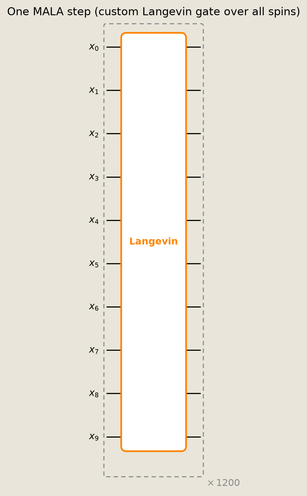
One step is a single custom gate acting on the whole dim-10 continuous pmode; HybridPCircuit repeats it reps times. The ten labeled coordinates are all components of that one pmode rather than ten separate sites, and the dense gate couples every coordinate through $\nabla V$.
fig = P_sch.draw_pcircuit(
    [("Langevin", list(range(n)))],
    wire_labels=[rf"$x_{{{i}}}$" for i in range(n)],
    title="One MALA step (custom Langevin gate over all spins)",
    reps=DEPLOY_REPS,
)
display_and_close(fig)
Validating against an exact reference
Because $\nabla V$ is nonlinear, the gate has no affine-Gaussian channel and no closed-form Gaussian moments to check against. We validate the sampler where the target is tractable instead: a single soft spin in the same quartic double-well with a field bias (the couplings switched off), whose Boltzmann density $\pi(x)\propto e^{-V(x)/T}$ we obtain by fine-grid quadrature.
This exercises the same sample code path as the graph run below (gradient drift plus, for MALA, the Metropolis accept/reject); only the energy coefficients differ. Matching the 1-D reference therefore validates the proposal-and-acceptance machinery against an exact target; the deployed 10-D chain, which has no tractable reference, is checked separately by long-run-MALA parity below.
To isolate the step-size bias from mixing, we hold the total simulated time $T_{\mathrm{sim}} = \texttt{reps}\times\varepsilon$ fixed across the sweep, so every chain integrates the same amount of dynamics and only the discretization changes.
LAM_1D = 1.5      # a stiffer well than the graph run, to make ULA's bias vivid
T_1D = 0.30
H_1D = 0.25
T_SIM = 60.0      # fixed simulated time; reps = T_sim / step isolates step-size bias
N_1D = 8000

EPS_SWEEP = [0.02, 0.06, 0.11, 0.16]
EPS_MATCH = 0.06  # step for the MALA-matches-reference panel
EPS_BIAS = 0.16   # step for the ULA-bias panel (the coarsest in the sweep)

grid = np.linspace(-3.0, 3.0, 1401)
The boltzmann_1d_reference helper evaluates the gate's own energy method on the grid and normalizes $e^{-V(x)/T}$ by quadrature, so the target we compare against is the same $V$ the gate descends.
ref_gate = LangevinGate(sites=0, dims=(1,), metropolis=True)
theta_1d = langevin_theta(
    adj=[[0.0]],
    field=[H_1D],
    beta=0.0,
    lam_quartic=LAM_1D,
    step=EPS_MATCH,
    temperature=T_1D,
)
ref_density, ref_cdf = boltzmann_1d_reference(ref_gate, theta_1d, grid)
We sweep the step size for both ULA and MALA, sampling N_1D independent chains at each $\varepsilon$ and scoring each empirical marginal against the exact reference with the ks_distance helper, a one-sample Kolmogorov-Smirnov statistic.
ula_1d, mala_1d = {}, {}
ks_ula, ks_mala = [], []
for eps in EPS_SWEEP:
    reps = round(T_SIM / eps)  # fixed simulated time T_sim = reps * eps
    theta_eps = langevin_theta(
        adj=[[0.0]],
        field=[H_1D],
        beta=0.0,
        lam_quartic=LAM_1D,
        step=eps,
        temperature=T_1D,
    )
    ula_1d[eps] = terminal_samples(
        theta_eps, metropolis=False, reps=reps, num_samples=N_1D, dim=1,
        key=jax.random.key(SEED + 100),
    )
    mala_1d[eps] = terminal_samples(
        theta_eps, metropolis=True, reps=reps, num_samples=N_1D, dim=1,
        key=jax.random.key(SEED + 200),
    )
    ks_ula.append(ks_distance(ula_1d[eps], grid, ref_cdf))
    ks_mala.append(ks_distance(mala_1d[eps], grid, ref_cdf))
for eps, ku, km in zip(EPS_SWEEP, ks_ula, ks_mala):
    print(f"eps={eps:.2f}  reps={round(T_SIM / eps):5d}  ULA KS={ku:.4f}   MALA KS={km:.4f}")

ks_match = ks_mala[EPS_SWEEP.index(EPS_MATCH)]
ks_bias_ula = ks_ula[EPS_SWEEP.index(EPS_BIAS)]
ks_bias_mala = ks_mala[EPS_SWEEP.index(EPS_BIAS)]

assert ks_match < 0.03, f"MALA does not match the reference: KS {ks_match:.4f}"
assert ks_bias_ula > 0.05, f"ULA bias not visible at eps={EPS_BIAS}: KS {ks_bias_ula:.4f}"
assert ks_bias_ula > 4 * ks_bias_mala, "MALA did not remove ULA's step-size bias"
assert ks_ula[-1] > ks_ula[0], "ULA KS should grow with the step size"
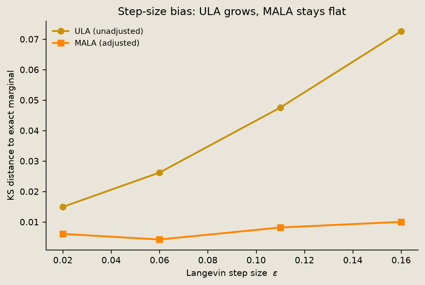
eps=0.02  reps= 3000  ULA KS=0.0150   MALA KS=0.0061
eps=0.06  reps= 1000  ULA KS=0.0262   MALA KS=0.0043
eps=0.11  reps=  545  ULA KS=0.0476   MALA KS=0.0082
eps=0.16  reps=  375  ULA KS=0.0726   MALA KS=0.0100
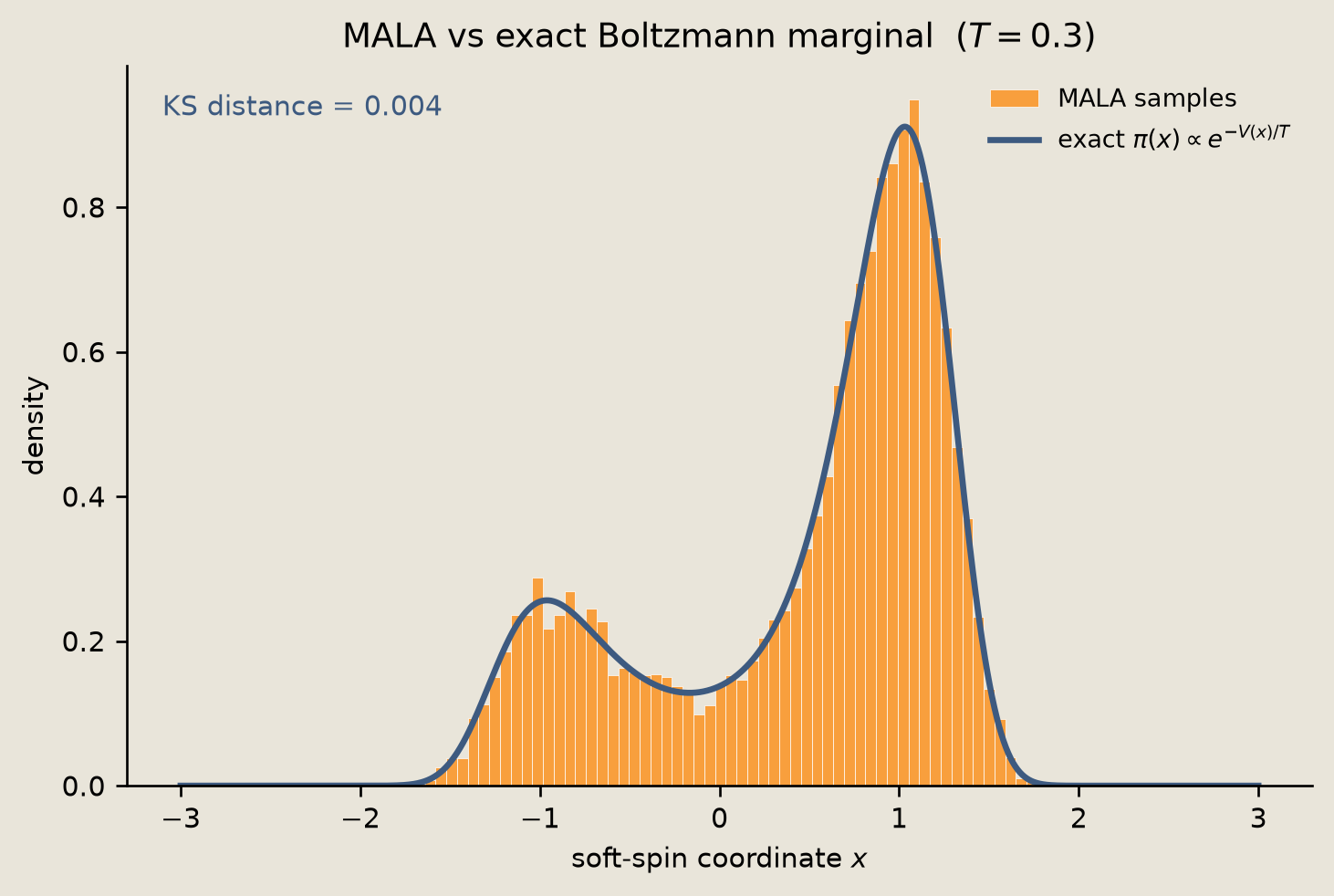
The MALA histogram sits on top of the exact Boltzmann density: with the accept/reject step, the chain samples $\pi(x)\propto e^{-V(x)/T}$ to within Monte Carlo noise.
fig = plot_mala_reference(
    grid, ref_density, mala_1d[EPS_MATCH], ks=ks_match, temperature=T_1D
)
savefig(fig, "12_langevin_mala_reference")
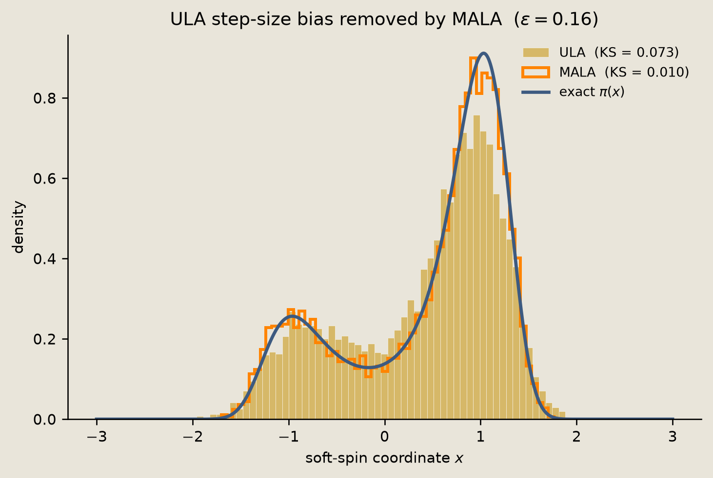
At a coarse step the unadjusted chain (ULA) underweights the main mode and overfills the trough relative to the exact density, while MALA, which runs the identical proposal plus accept/reject, stays on the target. That accept/reject step is what removes the bias.
fig = plot_ula_bias(
    grid,
    ref_density,
    ula_1d[EPS_BIAS],
    mala_1d[EPS_BIAS],
    step=EPS_BIAS,
    ks_ula=ks_bias_ula,
    ks_mala=ks_bias_mala,
)
savefig(fig, "12_langevin_ula_bias")
Across the step-size sweep, ULA's KS distance to the exact marginal grows with $\varepsilon$ (its $O(\varepsilon)$ discretization bias), while MALA stays flat near the Monte Carlo floor: the accept/reject correction holds at every step size.
fig = plot_ks_vs_step(EPS_SWEEP, ks_ula, ks_mala)
savefig(fig, "12_langevin_ks_vs_step")
Sampling the full graph
The 1-D checks validate the sampler's machinery on an exact target. We now deploy that gate on the full 10-node energy: NUM_SAMPLES independent chains, each DEPLOY_REPS Metropolis-adjusted steps from the zero state, returned in one JIT-compiled pass.
samples = terminal_samples(
    theta, metropolis=True, reps=DEPLOY_REPS, num_samples=NUM_SAMPLES, dim=n,
    key=jax.random.key(SEED),
)
assert samples.shape == (NUM_SAMPLES, n), f"expected ({NUM_SAMPLES}, {n}), got {samples.shape}"
assert np.all(np.isfinite(samples)), "non-finite samples"
print(f"samples shape: {samples.shape}  min={samples.min():.3f}  max={samples.max():.3f}")
samples shape: (1024, 10) min=-2.156 max=2.235
Is DEPLOY_REPS steps enough? With no tractable reference in ten dimensions, we compare per-site mean soft spins $\langle\tanh x_i\rangle$ against a much longer MALA run. Agreement within Monte Carlo error is a convergence sanity check: it is consistent with the deployed chain having reached the stationary law but does not prove it.
long_samples = terminal_samples(
    theta, metropolis=True, reps=LONGRUN_REPS, num_samples=NUM_SAMPLES, dim=n,
    key=jax.random.key(SEED + 1),
)
mu_deploy = np.mean(np.tanh(samples), axis=0)
mu_long = np.mean(np.tanh(long_samples), axis=0)

conv_err = float(np.max(np.abs(mu_deploy - mu_long)))
# Monte Carlo standard error of the per-site mean DIFFERENCE (two independent chains).
se_deploy = np.std(np.tanh(samples), axis=0) / np.sqrt(NUM_SAMPLES)
se_long = np.std(np.tanh(long_samples), axis=0) / np.sqrt(NUM_SAMPLES)
conv_se = float(np.max(np.sqrt(se_deploy**2 + se_long**2)))
print(f"deployed vs long-run per-site max abs diff = {conv_err:.4f}  (max MC SE ~ {conv_se:.4f})")
assert conv_err < 0.06, f"deployed MALA not converged: max abs diff {conv_err:.4f}"
deployed vs long-run per-site max abs diff = 0.0414 (max MC SE ~ 0.0309)
fig = plot_site_mean_parity(
    mu_deploy, mu_long, n=n, reps_short=DEPLOY_REPS, reps_long=LONGRUN_REPS
)
savefig(fig, "12_langevin_convergence_parity")
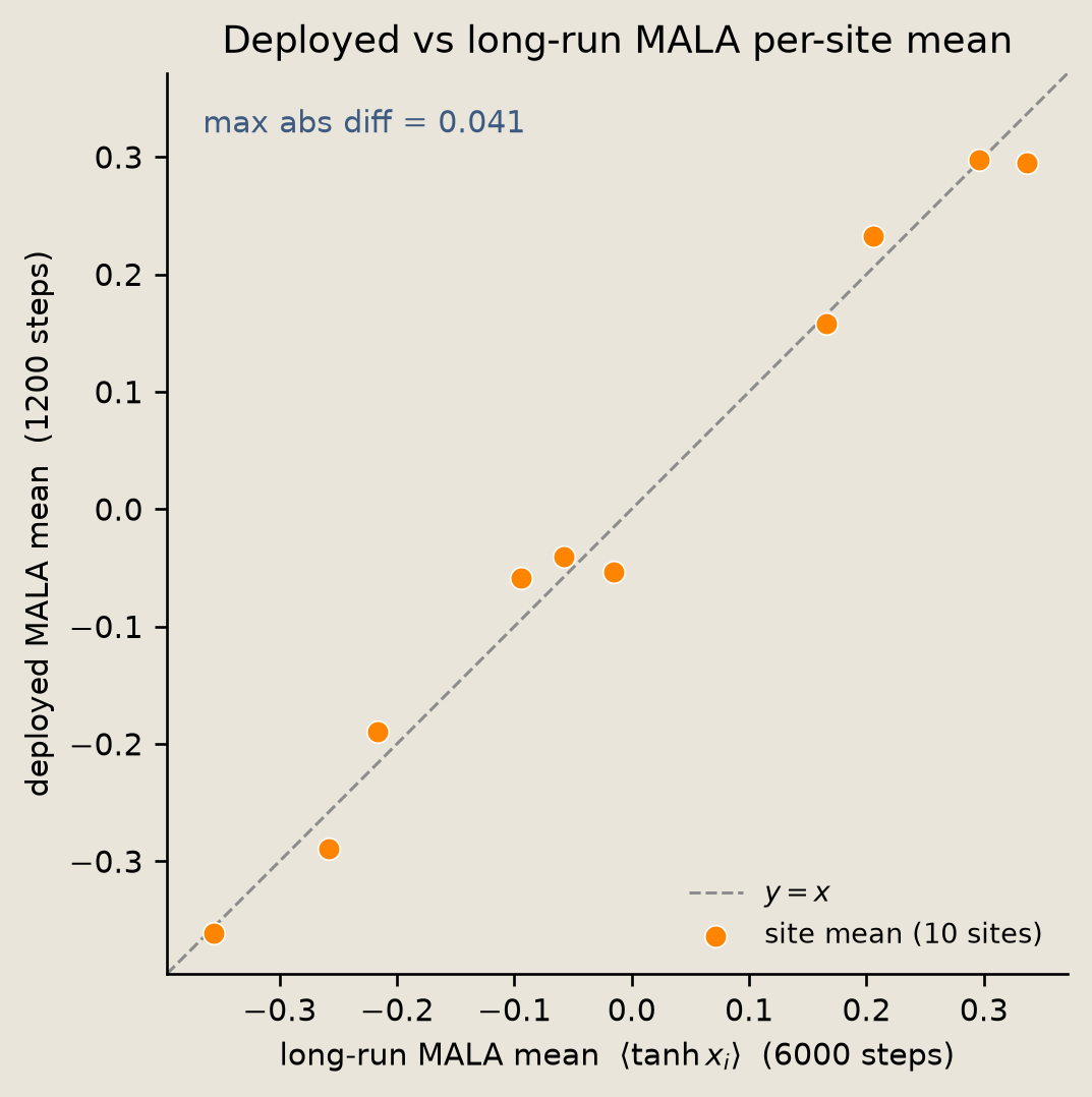
The deployed and long-run per-site means fall on the diagonal; the max per-site difference is about 1.3x the Monte Carlo standard error, consistent with convergence at this sample size.
Terminal field and magnetization
We summarize the terminal samples as a soft-spin field and a magnetization distribution.
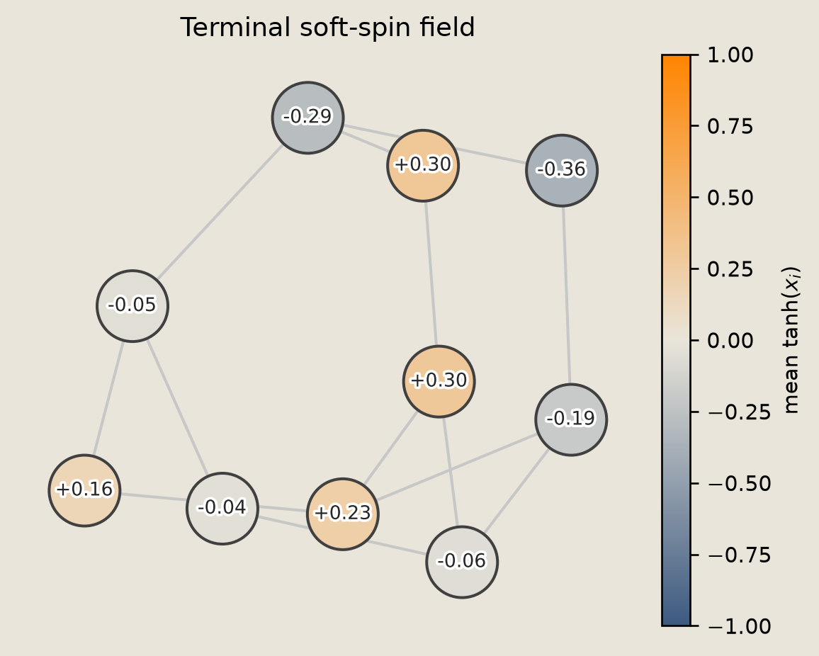
The graph view shows the mean soft spin $\tanh(x_i)$ over NUM_SAMPLES samples on the graph. A diverging colormap fits here because magnetization is signed.
We compute these summaries from the terminal states.
mean_soft_spin = np.mean(np.tanh(samples), axis=0)
terminal_magnetization = np.mean(np.tanh(samples), axis=1)
mean_mag = float(terminal_magnetization.mean())
The terminal field plot puts one labeled node at each graph site.
fig = P_sch.plot_terminal_field(graph, pos, mean_soft_spin)
savefig(fig, "12_langevin_terminal_field")
The magnetization histogram shows the per-path magnetization $m = \frac{1}{n}\sum_i \tanh(x_i)$ with the sample mean marked.
fig = P_samp.plot_magnetization_histogram_langevin(
    terminal_magnetization,
    title_hist=f"Magnetization distribution  ({NUM_SAMPLES} paths)",
)
savefig(fig, "12_langevin_magnetization")
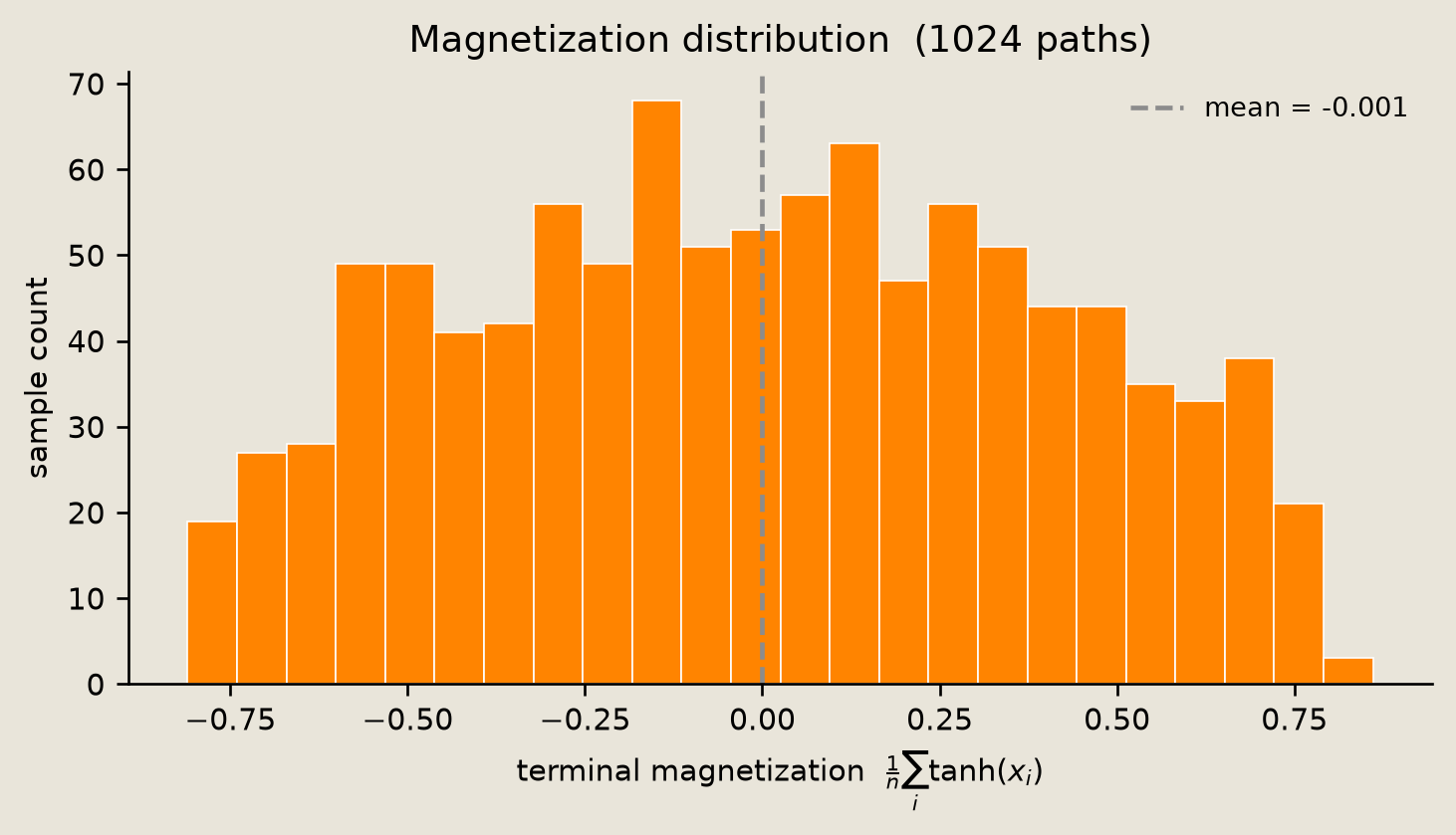
The external field is antisymmetric (it sums to about zero), so at equilibrium it induces per-site magnetization structure rather than a net polarization. The graph coloring above shows signed per-site structure consistent with the field, and the per-path magnetization distribution is broad but centered on zero (mean -0.001). These are equilibrium statistics of the Boltzmann law the gate samples, read from the converged terminal states.
Energy equilibration
A single MALA path scores its own energy $V(x_t)$ as it evolves. Starting from $x = 0$ every term except the quartic well vanishes, so $V(x_0) = \tfrac{\lambda_q}{4}\,n$. The energy then relaxes and fluctuates around an equilibrium band, the finite-temperature signature of Boltzmann sampling rather than descent to a single minimum.
We unroll one path with a compiled scan, recording $V(x_t)$ and the MALA acceptance rate along the way.
def run_mala_path(theta, *, dim, steps, key):
    """One MALA path: return (energies V(x_t) over the path, acceptance rate)."""
    gate = LangevinGate(sites=0, dims=(dim,), metropolis=True)

    def body(carry, _):
        x, k = carry
        k, subkey = jax.random.split(k)
        substate = {"discrete": jnp.zeros((0,), dtype=jnp.int32), "continuous": x}
        x_next = gate.sample(subkey, substate, theta)
        moved = jnp.any(jnp.abs(x_next - x) > 0.0)  # a rejection leaves x unchanged
        return (x_next, k), (x, moved)

    # one compiled scan unrolls the whole trajectory; no per-step host sync
    _, (path, moved) = eqx.filter_jit(
        lambda key: jax.lax.scan(body, (jnp.zeros(dim), key), None, length=steps)
    )(key)
    energies = jax.vmap(lambda x: gate.energy(x, theta))(path)
    return np.asarray(energies), float(np.mean(np.asarray(moved)))
TRACE_STEPS = 500
energies_arr, accept_rate = run_mala_path(
    theta, dim=n, steps=TRACE_STEPS, key=jax.random.key(SEED + 2)
)
assert np.all(np.isfinite(energies_arr)), "non-finite energy trace"

mean_energy = float(energies_arr.mean())
initial_energy = float(energies_arr[0])
tail_energy = float(energies_arr[-100:].mean())  # late-trace level shown in the figure and summary
fig = P_samp.plot_energy_trace(energies_arr, tail_energy)
savefig(fig, "12_langevin_energy_trace")
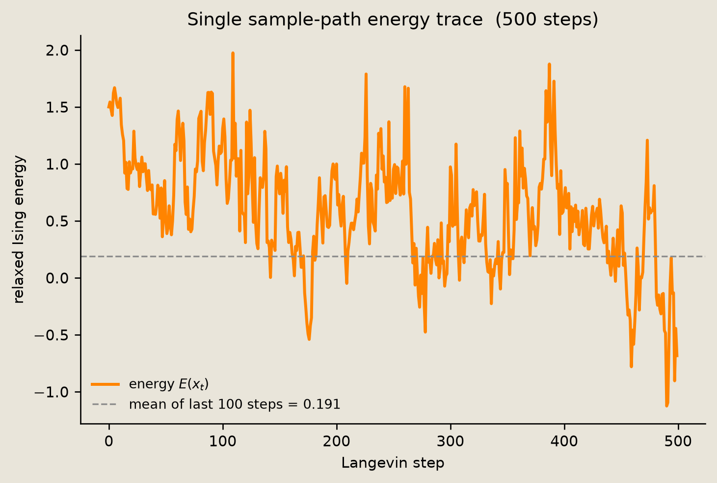
The energy drops from $V(x_0)$ and then fluctuates around a level well below the start, with fluctuations set by the temperature. The dashed line marks the mean of the last 100 steps, the same value the summary below prints; this single noisy path is still drifting slowly late in the trace, so we read the level as approximate.
Verification
We close with checks the earlier cells do not already cover: the MALA acceptance rate is healthy, the energy trace equilibrates well below its initial value, and the net magnetization is near zero. A summary block then prints the headline numbers.
assert accept_rate > 0.5, f"MALA acceptance too low: {accept_rate:.3f}"
assert np.isfinite(mean_energy), "mean energy is non-finite"
assert energies_arr.min() < initial_energy, "energy never descended below initial value"
assert tail_energy < initial_energy - 0.1 * abs(initial_energy), (
    f"energy did not equilibrate below the start: tail {tail_energy:.3f} vs "
    f"initial {initial_energy:.3f}"
)
assert abs(mean_mag) < 0.15, f"unexpected net polarization: mean magnetization {mean_mag:+.4f}"
print(f"-- Langevin graph Ising  (n={n}, deploy reps={DEPLOY_REPS}, {NUM_SAMPLES} paths) --")
print(f"  MALA acceptance rate  : {accept_rate:.3f}")
print(f"  deployed vs long-run  : max |d mean| = {conv_err:.4f}  (MC SE ~ {conv_se:.4f})")
print(f"  mean magnetization    : {mean_mag:+.4f}   (range [-1, 1])")
print(
    f"  magnetization range   : [{terminal_magnetization.min():+.3f}, {terminal_magnetization.max():+.3f}]"
)
print(f"  initial energy V(x_0) : {initial_energy:+.4f}")
print(f"  equilibrium energy    : {tail_energy:+.4f}  (mean of last 100 steps)")
print(f"  1-D MALA KS (eps={EPS_MATCH}): {ks_match:.4f}")
print(f"  1-D ULA  KS (eps={EPS_BIAS}): {ks_bias_ula:.4f}   (step-size bias MALA removes)")
print("--------------------------------------------------------")
-- Langevin graph Ising  (n=10, deploy reps=1200, 1024 paths) --
  MALA acceptance rate  : 0.974
  deployed vs long-run  : max |d mean| = 0.0414  (MC SE ~ 0.0309)
  mean magnetization    : -0.0008   (range [-1, 1])
  magnetization range   : [-0.810, +0.861]
  initial energy V(x_0) : +1.5000
  equilibrium energy    : +0.1910  (mean of last 100 steps)
  1-D MALA KS (eps=0.06): 0.0043
  1-D ULA  KS (eps=0.16): 0.0726   (step-size bias MALA removes)
--------------------------------------------------------
Conclusion
We sampled the continuous Boltzmann law of a soft-spin graph Ising energy with a custom LangevinGate.
The gate takes one gradient-drift step on $V$, with the gradient computed by jax.grad inside sample; HybridPCircuit repeats it and HybridSampleSimulator returns terminal states of independent chains in one JIT-compiled pass. On a tractable 1-D instance, the Metropolis-adjusted (MALA) chain matched the exact quadrature density; the step-size sweep quantified the unadjusted (ULA) bias it removes. Deployed on the full graph, MALA reached the same per-site statistics as a long-run reference, its energy equilibrated, and the soft-spin field showed the field-induced gradient.
Because the drift is nonlinear, the gate forfeits the closed-form affine-Gaussian moment simulator, so correctness is established by comparison to a tractable reference instead.
Next, 13_regime_switching_diffusion.ipynb drives a Gaussian process with a discrete control pdit.
References
- Roberts, G.O., Tweedie, R.L. 1996. Exponential convergence of Langevin distributions and their discrete approximations. Bernoulli 2(4), 341-363. Establishes that the Metropolis-adjusted Langevin algorithm converges to the target while the unadjusted discretization need not.
- Parisi, G. 1981. Correlation functions and computer simulations. Nuclear Physics B 180(3), 378-384. The Langevin-dynamics view of sampling a continuous field from its energy that the gate implements.